머신러닝의 첫걸음: NumPy와 Matplotlib로 선형회귀 데이터 시각화하고 분석하기

선형 회귀 모델(Linear Regression)의 기초적인 파이썬 코드 예제를 살펴보며 NumPy와 Matplotlib의 활용법을 배워보도록 하자.

 

코드 풀버전

import numpy as np
import matplotlib.pyplot as plt
plt.style.use('./deeplearning.mplstyle')

# x_train is the input variable (size in 1000 square feet)
# y_train is the target (price in 1000s of dollars)
x_train = np.array([1.0, 2.0])
y_train = np.array([300.0, 500.0])
print(f"x_train = {x_train}")
print(f"y_train = {y_train}")

# m is the number of training examples
print(f"x_train.shape: {x_train.shape}")
m = x_train.shape[0]
print(f"Number of training examples is: {m}")

# m is the number of training examples
m = len(x_train)
print(f"Number of training examples is: {m}")

i = 1 # Change this to 1 to see (x^1, y^1)

x_i = x_train[i]
y_i = y_train[i]
print(f"(x^({i}), y^({i})) = ({x_i}, {y_i})")

# Plot the data points
plt.scatter(x_train, y_train, marker='x', c='r')
# Set the title
plt.title("Housing Prices")
# Set the y-axis label
plt.ylabel('Price (in 1000s of dollars)')
# Set the x-axis label
plt.xlabel('Size (1000 sqft)')
plt.show()

---

 

코드 뜯어보기

 

import numpy as np

 

• NumPy 불러오기

NumPy는 숫자로 된 데이터들을 다룰 때 유용한 기능들을 모아 둔 수학 계산&데이터 처리용 도구 상자라고 할 수 있다. NumPy를 임포트하면 데이터 다차원 배열(e.g. 표), 수많은 숫자에 같은 연산 처리하기, 제곱근, 삼각함수, 로그 계산, 난수 생성 등의 기능을 사용 가능하다.

import numpy as np에서 as np는 넘파이 라이브러리를 간단하게 부르기 위해 축약형 이름을 np라고 정해준다는 뜻이다. NumPy 라이브러리 속 기능들을 사용할 때마다 일일이 NumPy를 타이핑하기 귀찮기 때문에 np라고만 쓰면 넘파이 라이브러리를 불러올 수 있다. 대부분의 파이썬 사용자들이 NumPy를 np로 부르는 걸 관례처럼 사용하기 때문에 다른 사람들이 np를 봐도 NumPy임을 이해할 수 있다.

 

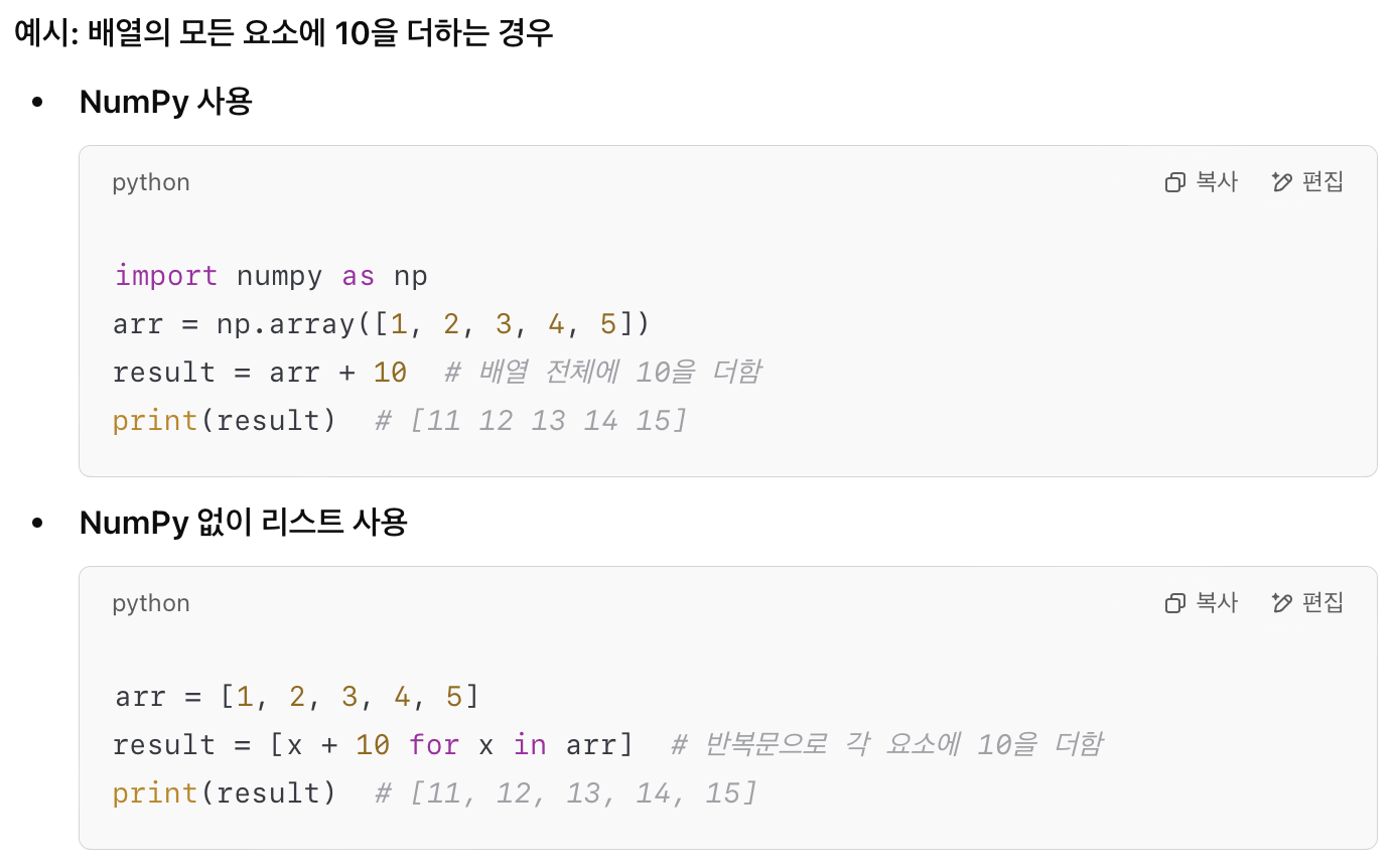
• 이 코드에서 NumPy 라이브러리를 불러온 이유

NumPy를 사용하면 배열 전체에 대해 한꺼번에 연산을 먹일 수 있다. 하지만 NumPy를 사용하지 않으면 반복문을 사용해 모든 데이터를 하나하나 계산해야 한다. 머신러닝의 경우 데이터 양이 많으므로 NumPy를 사용해야 계산이 오래 걸리지 않는다. 또한 for 반복문을 사용하지 않고 직관적으로 코드를 쓸 수 있어 편하다.

 

이 머신러닝 코드에서는 x 데이터셋과 y 데이터셋을 모두 트레이닝시켜야 하므로 다차원 배열이 필요하고, 데이터끼리 연산도 할 예정이다. NumPy를 사용하지 않고 리스트로 사용해도 1차원 배열뿐만 아니라 다차원 배열도 할 수 있다. 그리고 리스트로도 전체 데이터 개수를 확인할 수 있다(len()). 그러나 리스트는 단순히 데이터를 묶어 놓는 자료구조일 뿐, 배열 간의 수학적 연산은 지원하지 않는다. 그래서 리스트로 데이터를 정리할 경우 데이터끼리 계산을 할 때마다 수동으로 반복문을 돌려야 한다.

또한 넘파이는 다차원 배열의 행/열 정보 등 좀 더 다양한 정보들을 알 수 있다. 리스트는 단순히 요소들의 모음이라 데이터의 크기나 차원은 알기 어렵지만, NumPy는 .shape같은 속성을 사용해서 행열 정보도 알 수 있다.

---

import matplotlib.pyplot as plt

 

• pyplot 모듈 불러오기

Matplotlib라는 라이브러리의 pyplot 모듈을 불러오는 단계다. Pyplot은 Matplotlib의 일부다.

Mat는 대표적인 데이터 시각화 툴인 MATLAB(매트랩)에서 따온 것이고, Plot은 그래프(플롯)을 그린다는 뜻이다. lib는 Library의 약자다. 따라서 Matplotlib는 매트랩 느낌의 그래프그리기 라이브러리라는 뜻이다.

pyplot은 데이터를 그래프로 그려주는 도구들을 제공하며, 파이썬용 플롯 도구를 의미한다. Matplotlib의 Pyplot은 파이썬을 기반으로 동작하는 모듈이다. 'as plt'라고 한 것은 'as np'처럼 타이핑이 귀찮아서 약칭을 지정해 준 것이다. 이제 plt라고 쓰면 pyplot을 언급한 것이나 다름이 없다.

 

• pyplot 속 다양한 함수들

구분	함수명	함수 설명	사용 예시
데이터 시각화	.plot()	선형 그래프 그리기	plt.plot([1, 2, 3], [4, 5, 6])
	.scatter()	산점도(점 그래프) 생성	plt.scatter([1, 2, 3], [4, 5, 6])
	.bar()	막대 그래프 생성	plt.bar(['A', 'B', 'C'], [10, 15, 7])
	.hist()	히스토그램 생성 # 구간별 분포를 보는 막대그래프	plt.hist(data, bins=10) # bins는 데이터를 나눌 구간임
	.pie()	원형 그래프 생성	plt.pie([30, 50, 20], labels=['A', 'B', 'C'])
	.imshow()	2D 이미지 데이터 표시 # 히트맵 등	plt.imshow(2D 데이터 배열 이름, cmap='gray') # cmap은 데이터값을 색상으로 나타낼 때의 컬러맵. 색상 팔레트
	.boxplot()	박스 플롯 생성	plt.boxplot(data)
그래프 꾸미기	.title()	그래프 제목 설정	plt.title("그래프 이름")
	.xlabel()	x축 레이블 설정	plt.xlabel("x축 레이블 이름")
	.ylabel()	y축 레이블 설정	plt.ylabel("y축 레이블 이름")
	.xlim()	x축 범위 설정	plt.xlim(0, 10)
	.ylim()	y축 범위 설정	plt.ylim(0, 100)
	.legend()	범례 표시	plt.legend(['Line 1', 'Line 2'], loc='best') # 첫번째 변수는 범례 이름 지정. # 두번째 변수는 범례 위치 지정. 'best(알아서 예쁜 곳에)', upper right', 'lower left'등 입력 가능
	.grid()	격자선 추가	plt.grid(True)
데이터 스타일링	.style.use()	그래프 스타일 설정	plt.style.use('seaborn-darkgrid') # 'seaborn-darkgrid', 'seaborn-notebook', 'seaborn-white', 'ggplot', 'fivethirtyeight', 'dark_background', 'classic', 'bmh', 'Solarize_Light2' 등... # 직접 스타일을 만들어 .mplstyle 확장자 파일을 불러올 수 있음 # 스타일 초기화: plt.style.use('default')
	.color()	그래프 색상 설정	plt.plot(x, y, color='red') # 'blue', 'red', 'green', 'yellow', 'cyan', 'magenta', 'black', 'white' 가능 # RGB 색상 지정 가능 color=(0.5, 0.2, 0.8) # 헥사 코드 가능 color='#FF5733'
	.linestyle()	선 스타일 변경	plt.plot(x, y, linestyle='-')  # 실선 ─── plt.plot(x, y, linestyle='--')  # 점선 - - - - - - plt.plot(x, y, linestyle='-.')  # 점선-실선 혼합 ─‧─‧ plt.plot(x, y, linestyle=':')  # 작은 점선 .......
	.marker()	데이터 점 마커 설정	plt.plot(x, y, marker='o')
다중 그래프	.subplot()	여러 그래프를 한 화면에 배치	# (행, 열, 그래프 번호) plt.subplot(2, 1, 1)   # 위아래로 두개 배치한 거 중에 1번째 그래프라는 뜻 plt.plot(x1, y1) plt.subplot(2, 1, 2) # 위아래로 두개 배치한 거 중에 2번째 그래프라는 뜻 plt.plot(x2, y2)
	.figure()	새로운 그림 창 생성	plt.figure(figsize=(8, 6)) # 창 크기 지정 # 가로 8인치, 세로 6인치
데이터 표시 저장	.show()	그래프 표시	plt.show()
	.savefig()	그래프를 파일로 저장	plt.savefig("graph.png") # PNG 형식으로 저장 plt.savefig("graph.jpg", dpi=300)  # JPG 형식으로 저장 (해상도 300 DPI) plt.savefig("graph.gif")  # GIF 형식으로 저장 plt.savefig("graph.pdf")  # PDF 형식으로 저장 plt.savefig("graph.svg")  # SVG 형식으로 저장
텍스트 추가	.annotate()	데이터 점에 화살표 주석 추가	# plt.annotate(text, xy, xytext, arrowprops) # text: 주석에 표시할 텍스트 # xy: 화살표가 가리킬 점의 x,y좌표 # xytext: 주석 텍스트가 표시될 x,y 위치 # arrowprops: 화살표 스타일 정의. shrink는 화살표 길이 plt.annotate('Important point', xy=(2, 3), xytext=(3, 4),              arrowprops=dict(facecolor='black', shrink=0.05))
	.text()	그래프에 텍스트 추가	plt.text(2, 3, 'Label') # 그래프의 좌표 (2, 3)에 Label이라는 글자를 추가하겠다는 뜻 # 2차원 배열의 2행 3열 데이터에 글자를 쓰겠다는 의미 아님

 

---

plt.style.use('./deeplearning.mplstyle')

위 표에 따르면 이 코드는 사용자 정의 스타일 파일(.mplstyle)을 불러와 표를 꾸미는 코드다. mpstyle은 Matplot Style의 약자다.

---

x_train = np.array([1.0, 2.0])
y_train = np.array([300.0, 500.0])

x_train이라는 새로운 변수를 만들었고, 여기에 NumPy의 .array()를 사용해 1차원 배열을 생성했다. 마찬가지로 또 다른 변수 y_train을 만들어 여기에도 1차원 배열을 넣었다.

배열	x_train[0]	x_train[1]
x_train	1.0	2.0

 

배열	y_train[0]	y_train[1]
y_train	300.0	500.0

 

---

print(f"x_train = {x_train}")
print(f"y_train = {y_train}")

 

• 파이썬에서 print() 함수 사용법

print()의 괄호 안에는 문자열 형식만 들어가야 한다. 문자열과 변수를 같이 쓰고 싶다면 f"..." 형식의 f-string을 활용해야 한다. f"..."안에는 변수가 들어가도 최종적으로는 문자열로 반환해준다.

중괄호{}는 f-string 안에서 변수나 표현식을 삽입할 때 사용한다. 변수인 y_train의 값이 중괄호 {}안에 삽입되어 문자열 형식으로 출력되는 것이다. 

• f-string의 활용 예시

x = 5
y = 10
print(f"The sum of {x} and {y} is {x + y}")  # The sum of 5 and 10 is 15